🧑🏻‍🤝‍🧑🏽 HR Analysis: Predicting Employee Turnover with Machine Learning (EDA, Regression, Tree Based Models & XGBoost) - Full Process

Image Source: peoplemanagingpeople.com

Data Science Process

In this project, the following skills were applied: Cleaning, EDA, Machine Learning Models (Logistic Regression, Decision Tree, Random Forest) and Recommendations

Please use the outline on the right side of the webpage for easier navigation!

Project Objective Overview

• Central Question: Why causes employees to leave the company?
• We are tasked to understand the employee turn over in the company.
• Based on this, we pull insights and strategical recommendations.
• Libraries used include: numpy, pandas, matplotlib, seaborn, sklearn (logistic regression, decision tree, random forest, gridsearch, metrics) and pickle to save the model.
• You can access the Jupyter Notebook IPYNB file here LINK
• Access the raw dataset used here LINK
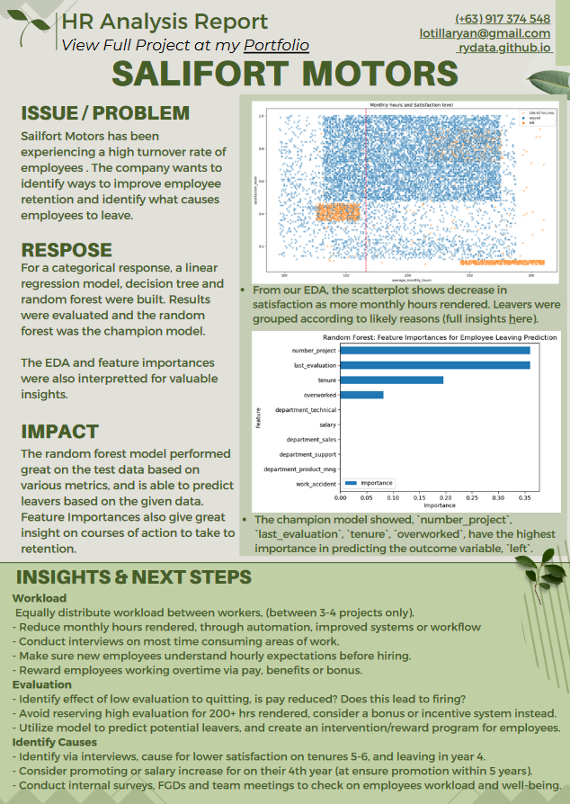
• Access the 1 Page Report summarizing projects insights here GDRIVE LINK

Project Findings Overview

On Employees who stayed:

• Staying employees had an average of 3-4 projects assigned, rendering monthly hours of 150-255 (still high compared to average of 167hrs)
• Satisfaction levels were generally high but lowered for tenure/years 5-6.

On Employees who left:

• Employees are generally overworked with almost double the regular monthly hours.
• Those who left either worked less hours and had only 2 projects assigned OR
• Are overworked with 255 - 300+ hours and had had more projects (4-7 projs assigned).
• Everyone with 7 projects assigned left.
• Highly satisfied employees, with more than 5 years are leaving due to lack of promotion and salary increase.
• Those with 4 years in the company, may have left due to drastic policy change.

On Regression and Machine Learning Models:

• The logistic regression model approach achieved high scores (79% precision, 82% recall, and f1 of 80%).
• The decision tree model and random forest had even better scores and performed similarly (94% precision, 91% recall, f1 of 93%, accuracy and auc 98%).
• Feature Engineering was used to drop data which will not be realistically available.
• Second round of tree models were created. The random forest is the champion model and scored very well on the test set: (87% precision, 91% recall, 89% f1, accuracy 96% and auc 94%)

Recommendations at the end!

Data Cleaning and Preparation

Here is what the first 5 rows of our dataset looks like:

	satisfaction_level	last_evaluation	number_project	average_montly_hours	time_spend_company	Work_accident	left	promotion_last_5years	Department	salary
0	0.38	0.53	2	157	3	0	1	0	sales	low
1	0.80	0.86	5	262	6	0	1	0	sales	medium
2	0.11	0.88	7	272	4	0	1	0	sales	medium
3	0.72	0.87	5	223	5	0	1	0	sales	low
4	0.37	0.52	2	159	3	0	1	0	sales	low

• In total, our dataset contains 10 columns and 14999 rows of data on the employees. All insights and findings will be solely derived from this data set.
• Again, you may access the raw dataset used here LINK

After importing the packages we can do our initial data cleaning:

• head(), .info, .describe and .columns to better understand our data
• rename the columns to snake_case (lowercase and underscores) and correct mispellings
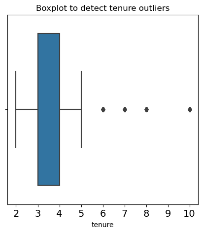
• .isnull(), .duplicated(), .drop_duplicates() to check for missing values and duplicates
• boxplot to check for outliers

We use Interquantile Range to identify the outliers. Fortunately there were no null values, however, there were about 3000 duplicates and 824 outliers in the tenure section. There are no major ethical considerations at this stage however we need to consider whether or not to remove outliers.

EDA and Visualization

Using the .value_counts(normalize=True) function, we can see the ratio of leavers. 1991(17%) left and 10000(83%) stayed.

Data Visualizations

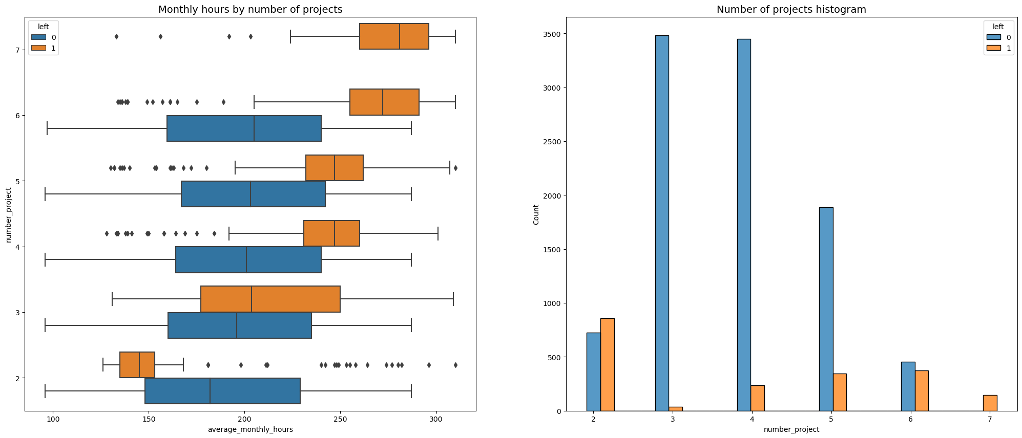
First, we use a stacked boxplot from the seaborn library to show the average monthly hours, compared to number of projects. We used stacked to visualize those who left (marked as 1) and those stayed (marked 2).

1. Monthly Hours by Number of Projects (Stacked Box plot)

From here we can observe that leavers fall into certain groups ff:

Group A:

• Assigned only 1-2 projects, this has the highest amount of leaves. These group worked significantly less hours than peers.
• It is possible these were fired due to lack of hours, or were assigned less since they have filed LOA, vacation or leave notices.

Group B:

• Assigned 4-7 projects, as projects increase, so does monthly hours, and leaves.
• Everyone assigned 7 projects left.
• Worked significantly more hours and are overworked.
• Worked 255 - 295 hours for a month. Double the usual amount of 166 hours (8 hrs, 5x a week, 4x a month).

Stayed Group:

• Assigned 3-4 projects, working 150 - 255 hours, had the highest amount of stays.
• Compared to the average 166 hours, this group still works a significant amount of hours.

2. Monthly Hours and Satisfaction level (Scatter Plot)

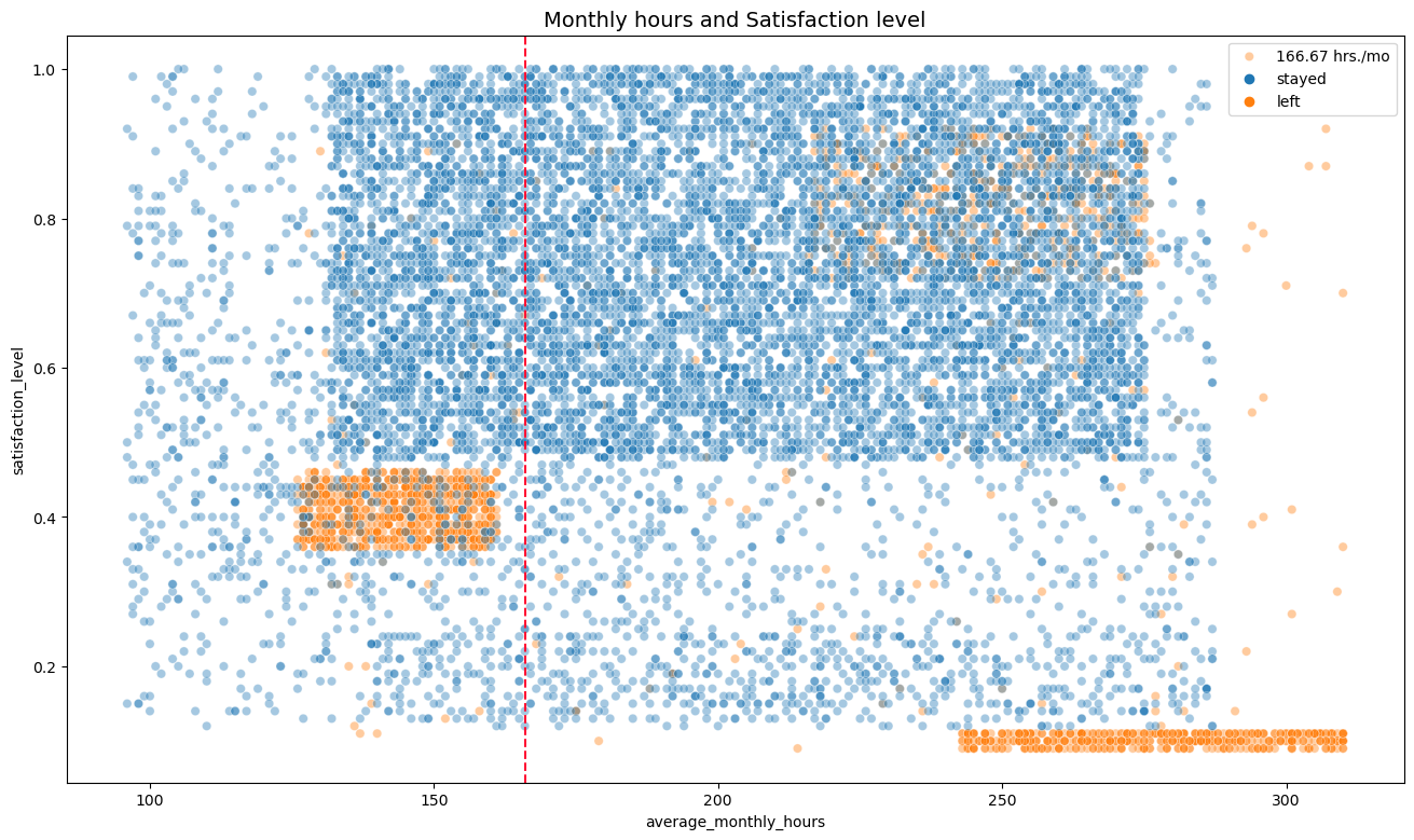
• This scatter plot examines average monthly hours and satisfaction levels.
• The dotted red line shows us a reference point of an average 166 hours for the average employee hours.
• Notice how leavers (in orange) are clumped in certain areas of the scatter plot. This backs up our observation on Group A and Group B as mentioned earlier.
• Group C: Looking at the top right of the plot, we notice a third group not evident in the first box plot.
  • This group has high satisfaction (0.8) but paired with high work hours (225-275), ended up leaving.

Note that we also see a strange shape of distribution, showing signs of synthetic data as distributions are not evenly distributed but instead are clumped up. They are also skewed to the right.

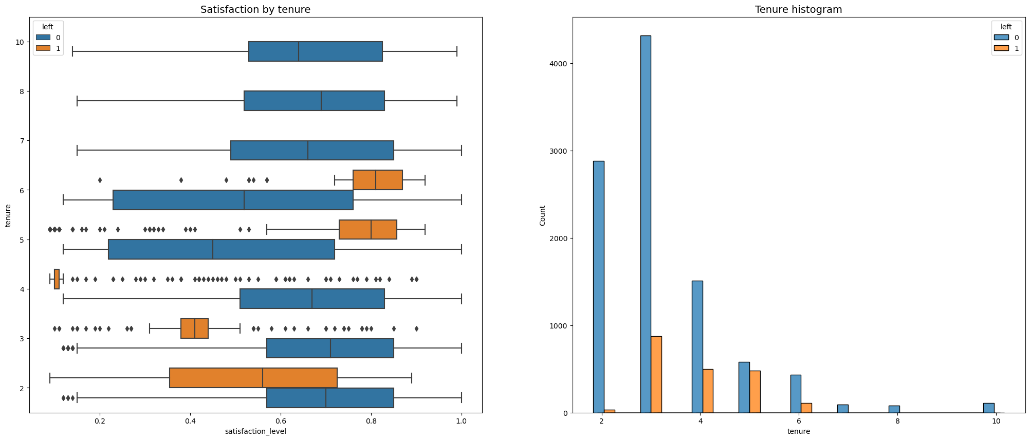
3. Satisfaction by Tenure (Stacked Box plot)

Let’s continue using our grouping system to make general observations. We can compile them later. From this visual we can observe the ff:

• 2 years had generally low satisfaction (Group D)
• 3 years had low satisfaction and highest leaves (Group D)
• 4 years has set of dissatisfied employees who left (Group F)
• 5-6 years had high satisfaction, but left (Group E)

Employees who left fell into two categories:

• Group D. Dissatisfied with lower tenures and
• Group E. Very satisfied with medium to higher tenures.
  • Further investigation should be done. Why did the employees leave despite a high amount of satisfaction?
  • It is possible that although they enjoyed their work, lack of promotions or salary increase caused them to leave.
• Group F. 4 Year tenure, with very low satisfaction.
  • It is worth investigating further that led to very low dissatisfaction levels. Did this group face major changes in policies or salaries?
• Satisfaction levels of year 7-10 and new employees are similar. Looking into which reasons led them to stay will be valuable.

A closer look will be applied for Group E as it is questionable why they left despite high satisfaction.

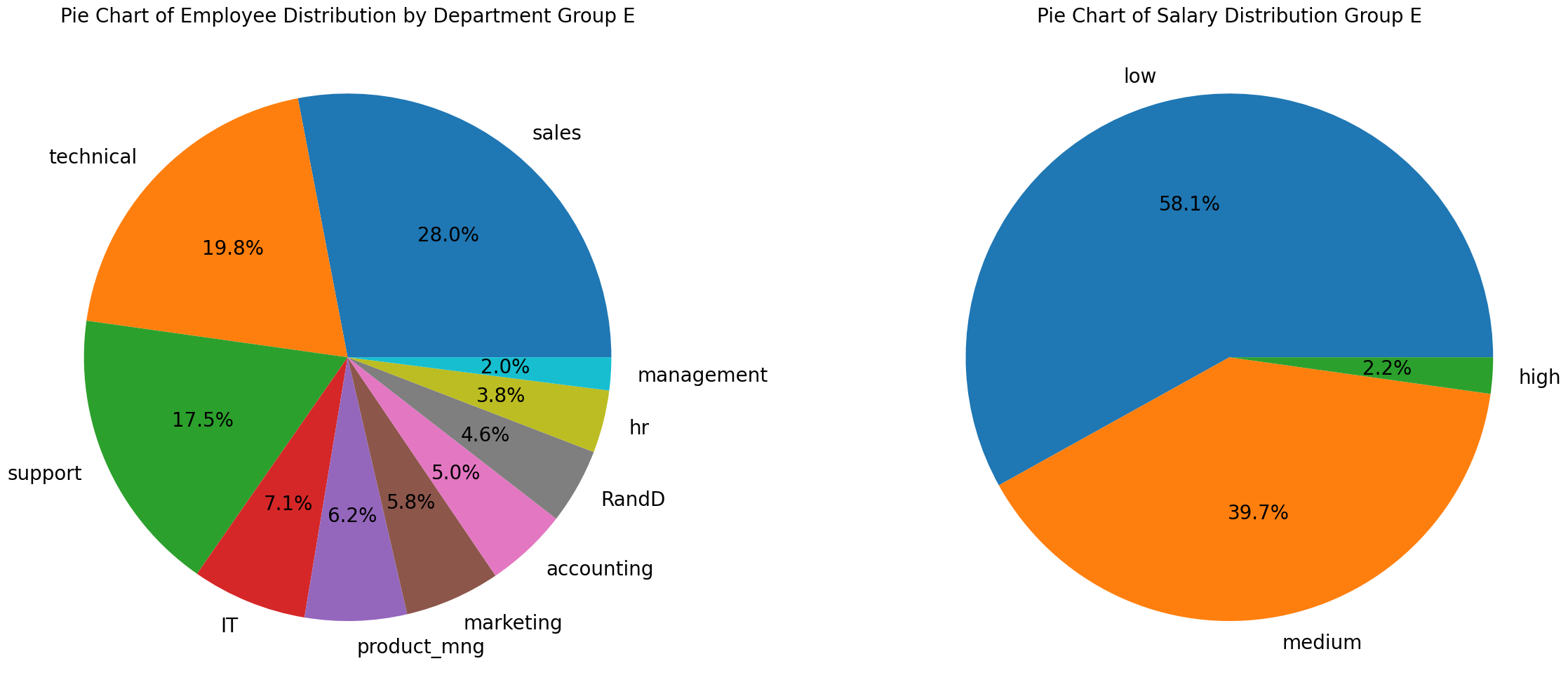
4. Group E: Employee and Salary Distribution (Pie Chart)

• To analyze this we filtered the group by satisfaction level of 7 or more, tenure of more than 5 and left the company.
• Despite being in the company for 7+ years, only 2% had high salaries. 58% have low salaries, and the rest are in medium.

• 28% are in sales, 19% in IT and 17% in support. Only 1 person was promoted.

• Despite the high satisfaction, leaves may be caused by lack of promotion and increase in salary despite the amount of years in the company.

5. Mean and Median Analysis on Leaves and Stays (Table)

• We use this code block to show a table depicting the mean and median satisfaction of employees who left and stayed:

# Calculate mean and median satisfaction scores of left and stayed
df1.groupby(['left'])['satisfaction_level'].agg([np.mean,np.median])

	Mean	Median
Left	0.677	0.69
Stayed	0.440	0.41

For those who stayed (Mean < Median):

• Distribution is negatively skewed
• There are more extreme scores (dissatisfied) in the bottom than at the top (satisfied)
• The majority are only moderately satisfied, but there is a small number very dissatisfied pulling down the mean.
• The company may have a polarized environment - meaning there are very satisfied and very dissatisfied workforce

For those who left (Mean > Median):

• The most dissatisfied employees are more likely to leave, the company looses its unhappiest employees, improving overall satisfaction in remaining, this may be a flag of high turn over rates.
• There are root issues not addressed leaving to more leaves.

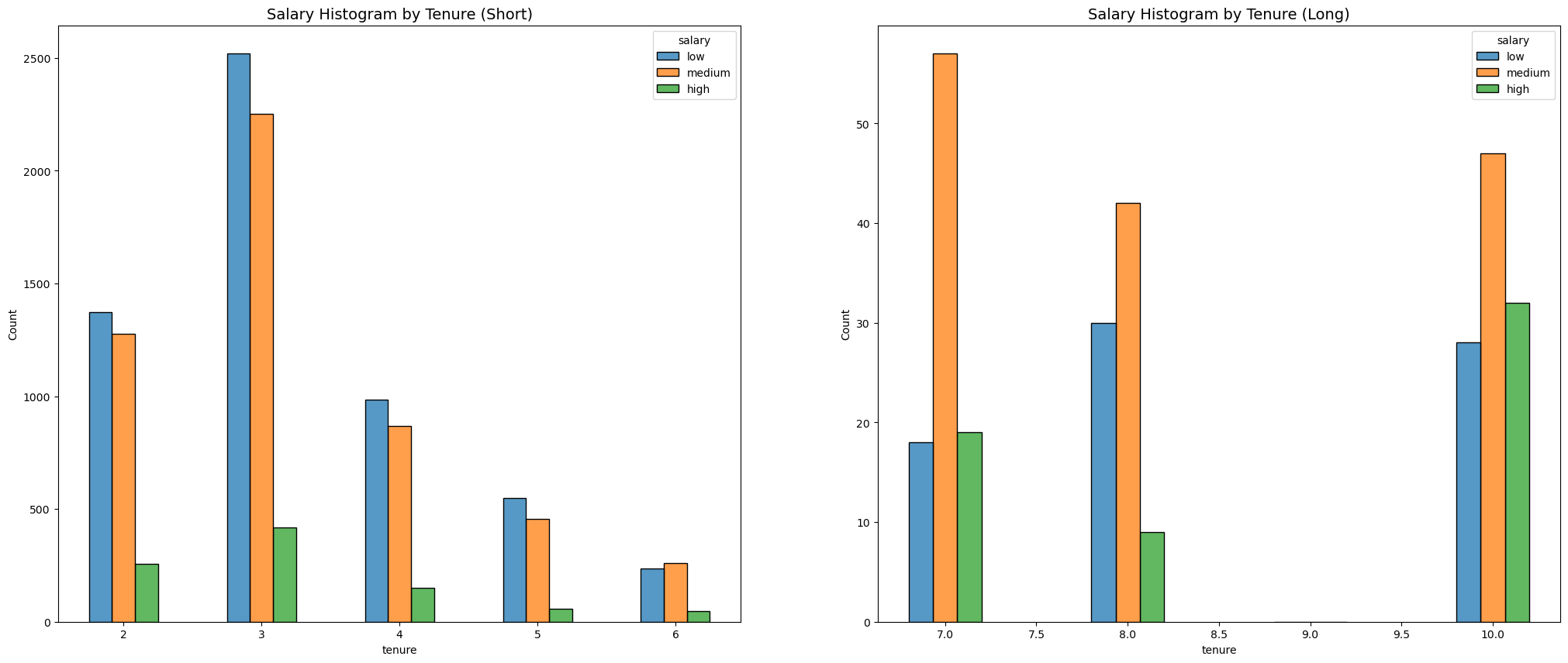
6. Salary Histogram by Tenure (Short and Long, Histogram)

• As years increase, the salary does not increase proportionally.
• Longer years did not necessarily convert to higher salary.
• For those that are paid high salaries, they have stayed in the company for more than 10 years. This may refer to C-level managers.

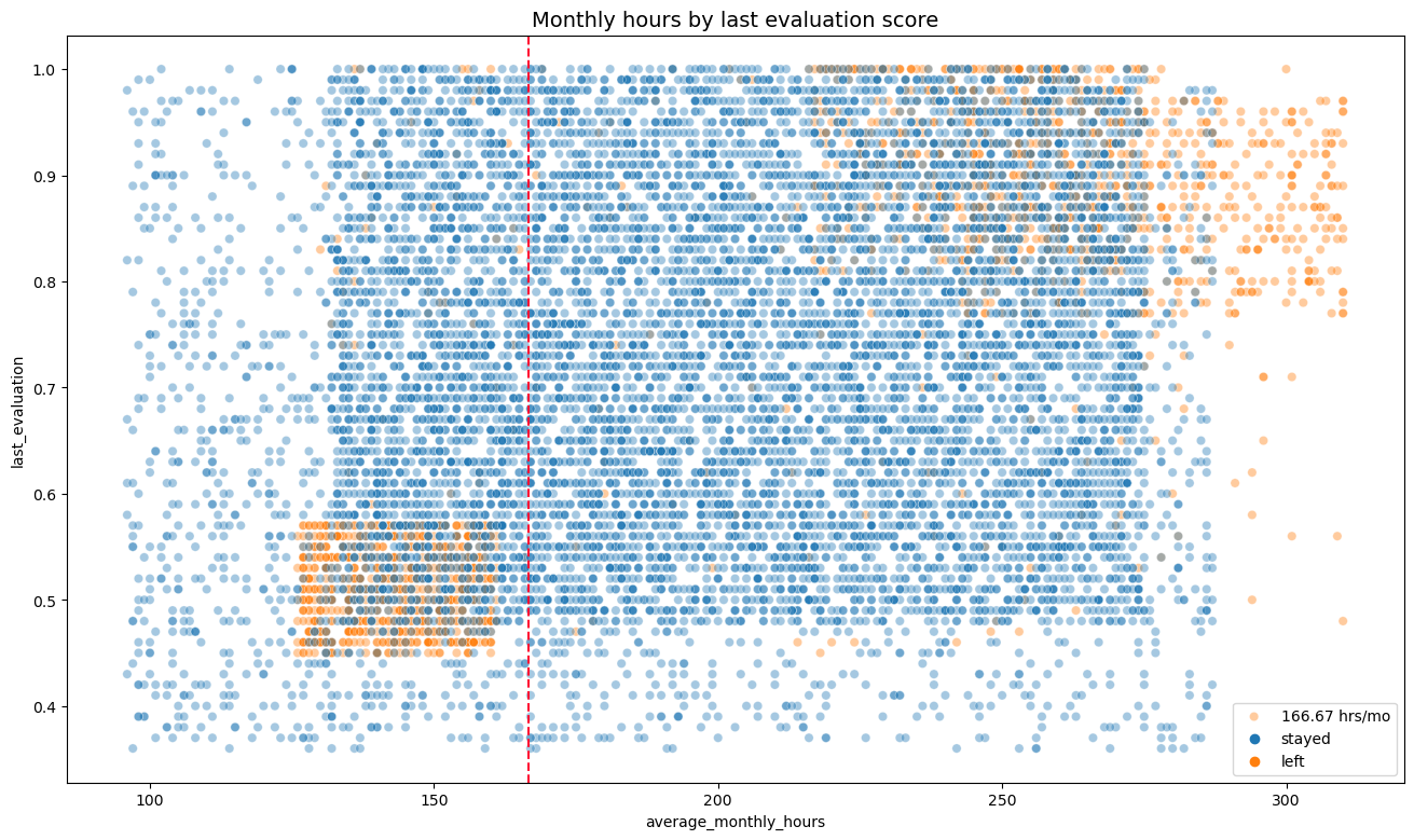
7. Monthly hours by evaluation score (Scatter Plot)

• Leavers (orange) are observed in the lower left and upper right of the plot.
• Two leave groups can be found again:
  • High monthly hours and received high evaluation
  • Less time below the average monthly hours and received low evaluation
• Working long hours does not guarantee high evaluation score since evaluation is still distributed randomly across increasing hours
• Again, large majority of employees work more than 167 hours a month.

8. Monthly hours by promotion (Past 5 years, Scatter Plot)

The plot informs us the following:

• The top part shows those who received promotions. Those below did not.
• The proportion of promoted in the last 5 years were small in relation to the amount of employees.
• Most of those who left were from those not promoted, despite working the longest hours.

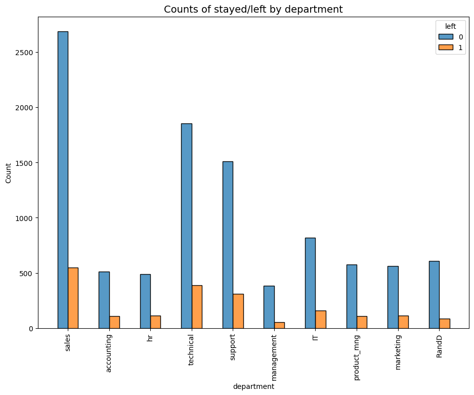
9. Employee Leaves by Department (Histogram)

• No department in particular has a proportionally amount who stayed or left.
• Although, sales, technical and support has the highest amount who left - this is balanced by the fact that there are more employees as well.

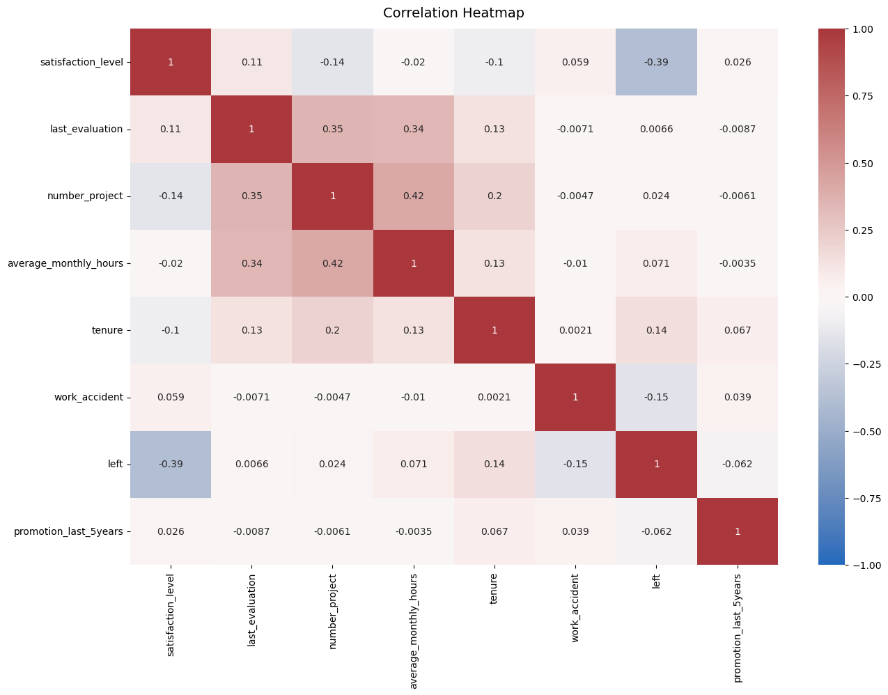
10. Variable Correlation (Heatmap)

The highest positive correlation includes:

• Number of projects and average monthly hours
• Last evaluation and number of projects
• Last evaluation and average monthly hours

The highest negative correlation includes:

• satisfaction level and employees left

EDA Insight Summary!

Various observations can be said through our eda, we found that leaving is related with:

• longer working hours
• increasing amount of projects
• lower satisfaction levels
• lack of promotion
• lack of increase in salary throughout years.

Working long hours, but not receiving promotions, higher salary, or better evaluation scores may have caused dissatisfaction and burn out. Despite this, people who have stayed for more than 6 years tend to stay.

Expand for additional insights:

To decrease confusion of our alphabetical groupings, we will compile them into 4 main categories of “Churned”.

Churned 1 includes:

• Group A: Significantly worked less hours with only 2 projects assigned
• Group D: dissatisfied and with lower tenure, 3 years and below
• This subgroup have lower tenures, worked less hours and had less projects assigned.

Churned 2 includes:

• Group B: Significantly more hours worked and more projects assigned
• Everyone with 7 projects assigned left
• This subgroup may have been exposed to overwork or experienced burnout.

Churned 3 includes:

• Group C: High satisfaction, but very significant amount of work hours 225 - 275.
• Group E: High satisfaction, with higher tenure (more than 5 years) but still left
• This subgroup may have left due to lack in promotion and salary increase.

Churned 4 includes:

• Group F: 4 Year tenure with very low satisfaction
• This subgroup may have experienced impactful changes.
• Further investigation of changes in policies required.

Stayed:

• For the groups who stayed, there was an average of 3-4 projects assigned.
• High monthly hours of 150-255 hours, from the average 166.7
• Satisfaction level ranges were relatively high for tenures 2-4, lowered for tenures 5-6, then returned to the initial ranges for 7 and above years.

Model Building A - Logistic Regression 🧪 📈

The following is a concise outline of steps taken, however, we will not be going into detail.

Again, feel free to visit the jupyter notebook for step by step information here LINK

Expand for Steps Taken:

1. Encode non-numeric variables (via pd.get_dummies function)
2. Correlation Heatmap
3. Employees Left / Stayed across Depts.
4. Remove outliers
5. Feature Selection
6. Test, train split
7. Fitting the model
8. Confusion Matrix
9. Checking class balance
10. Evaluation of Metrics

Logistic Regression Model Evaluation

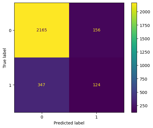
To evaluate a model we can use a Confusion Matrix to show us the amount of True Positives/Negatives and False Positives/Negatives

Correct Predictions:

1. Top Left: True Positives - Predicted leaving and actually left.
2. Lower Right: True Negatives - Predicted staying and actually stayed.

False Predictions:

1. Top Right: False Positives - Predicted leaving but stayed
2. Lower Left: False Negatives - Predicted staying but left.

What this means

• The model was able to correctly predict the majority of employees leaving (2165).
• The next largest quadrant is False Negatives, meaning the model predicted leavers, who actually stayed.
• This means that our model has a little bit of overfitting, as it is sensitive to factors that would make employees leave, this is good since the model is sensitive to employee that has potential to leave.

Scoring

• With 83% and 17% split, the balance is not perfect, but not too imbalanced also, this may have cause the slight overfit.

• Due to this accuracy is not a good metric, but we can use precision, recall, f1 and support.

• The logistic regression achieved a precision of 79%, recall of 82%, and f1 of 80%.

Model Building B - Decision Tree and Random Forest ⚗️🏕️

The following is a outline of steps taken throughout the Decision Tree modeling. For full steps visit the jupyter notebook here LINK

1. Isolate Dependent Variables
2. Select Features
3. Test Training Split

Decision Tree 1 🌲

Expand for Steps Taken

1. Instantiate, Params, Scoring and GridSearch
2. Fit Model
3. Best Params and AUC
4. Extract Scores

Scores:

• 92% Precision, 92% recall, 92% F1, 97% accuracy and auc.
• All scores are past 90% which are VERY strong indicators of a good model.
• We will also build a random forest to reduce overfitting, and grid search for the best parameters.

Random Forest 1 🏕️

Expand for Steps Taken

1. Instantiate, Params, Scoring and GridSearch
2. Fit Decision tree model to training data
3. Save model via Pickle
4. Best Params, AUC and Evaluate Scores
5. Get all scores
6. Pickle to save model training time

Scores:

• This model performed outperformed the decision tree model.
  • 95% Precision, 92% recall, 93% F1, 98% accuracy and auc.
• As the better model, let’s use our test set here. Our test set is a portion of the data that we hide, so we can use it to evaluate our model after training it.
• Test set scoring:
  • 96% Precision, 92% recall, 94% F1, 98% accuracy and 96% auc.
  • Our model performed even better in the test set.
  • We can be confident that the model will perform well on unseen data.

Feature Engineering for 2nd round of Modeling

• Our evaluation scores seem to high and may be cause by data leakage.
• This happens when we use data which may:
  • Already exist in test data
  • Realistically, we may not have access to this data during deployment
• During HR’s daily operations, we may not have immediate access to satisfaction levels.
• Average monthly hours may also be too correlated if employees already gave a resignation notice.
• Lets apply the ff:
  1. Satisfaction level column is removed
  2. New column ‘overworked’ will be either 1 (for 175 hrs+ rendered) or 0 (less than 175 hrs).
  3. Isolate new variables
  4. Create test, train split.

Decision Tree 2 🌲🌲

Based on our new features, let’s create a second decision tree.

Expand for Steps Taken

1. Instantiate, Params, Scoring and Grid Search
2. Fit model to values
3. Best Params, Best scores

Scores:

• The model has great performance despite dropping satisfaction levels and detailed work hours.

model	precision	recall	F1	accuracy	auc
Decision Tree 1 CV	91.46%	91.69%	91.57%	97.20%	96.98%
Decision Tree 2 CV	85.67%	90.36%	87.89%	95.85%	95.94%

Random Forest 2 🏕️🏕️

We will also create a 2nd random forest based on our new features.

Expand for Steps Taken

1. Instantiate, Params, Scoring and Grid Search
2. Fit model to values
3. Pickle
4. Best Params, Best scores, make results
5. Confusion Matrix

Scores:

• As expected, scores lowered with dropped values, however model still works great.

model	precision	recall	F1	accuracy	auc
Decision Tree 1 CV	91.46%	91.69%	91.57%	97.20%	96.98%
Random Forest 1 CV	94.87%	91.56%	93.18%	97.78%	98.04%
Decision Tree 2 CV	85.67%	90.36%	87.89%	95.85%	95.94%
Random Forest 2 CV	86.64%	88.08%	87.32%	95.76%	96.49%

• If AUC is our deciding matrix, random forest 2 performed better.
  • AUC is useful in our situation some with class imbalance
  • It is also a good metric when comparing ranking different models.
  • Random forest 2 is our champion model 👑

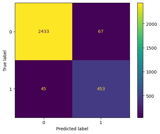
Lets evaluate the model with our test set and create a confusion matrix.

model	precision	recall	F1	accuracy	auc
Random Forest 2 CV	87.12%	90.96%	89.00%	96.26%	94.14%

Recall that:

1. Top Left: True Positives - Predicted leaving and actually left.
2. Lower Right: True Negatives - Predicted staying and actually stayed.
3. Top Right: False Positives - Predicted leaving but stayed
4. Lower Left: False Negatives - Predicted staying but left.

• The model was able to correctly predict the majority of employees leaving (2433).
• The next largest quadrant is the True Negatives, meaning the model predicted stays successfully.
• Since our model predicted more false positives than false negatives, it is likely to predict leavers, who actually stay. This is good since our model is sensitive to leavers.
• Compared to our Linear regression model, this has significantly better performance.

Decision Tree Splits and Feature Importances

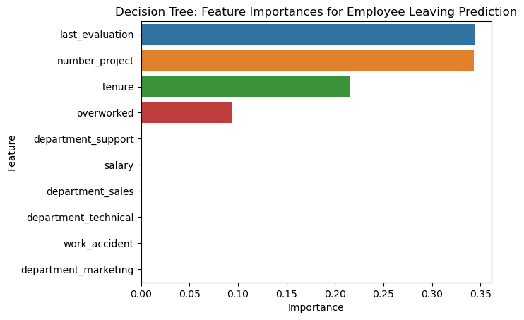
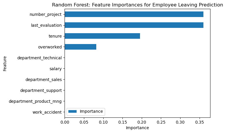
This graph shows the decision tree splits, although a bit cluttered, we can use Feature Importances with a barplot to see which variables were most important in prediction.

Decision Tree: Feature Importances for Employee Leaving Prediction

Random Forest: Feature Importances for Employee Leaving Prediction

We can see that he most important predictors on leavers are:

1. Number of Projects assigned
2. Last Evaluation (Ranked first in Decision Tree)
3. Tenure
4. Overworked

What this means:

1. Although further investigation is needed, we see that the last evaluation is one of the top predictors.
   • This means that employees are severely impacted by their performance review, or
   • Low performance reviews eventually lead to leaving:
     • whether by resignation, firing, lower pay or other factors.
2. Number of projects assigned and overwork are also both top predictors, our earlier findings our supported.
3. Finally tenure is also one of the most important predictors.
   • It is important to conduct interviews or follow-up investigation on the groups of individuals that left the company (such as year 4 leavers).

Recommendations and Next Steps for Salifort Motors

Expand for Full Summary/Recap in earlier stages

Insights Based on Model

Findings from EDA

Leaving is related to:

• longer working hours
• increasing amount of projects
• lower satisfaction levels
• lack of promotion
• lack of increase in salary throughout years

The leavers fall into the ff groups:

1. Worked less hours and only 2 projects assigned, lower tenures 3 and below
2. Worked more hours and more projects assigned, (7+ assigned all left)
3. High satisfaction, but high amount of work hours, lack of promotion or salary increase
4. Tenure of 4 years, may have experienced impactful changes.

Here are the attributes of those who stayed:

1. Average of 3-4 projects assigned
2. Monthly hours rendered 150-255
3. High satisfaction for tenure 2-4, lower for 5-6 and reaches initial ranges 7 on above.

Findings from Modeling

From the importance features the ff were identified as top leaving predictors:

1. Number of Projects assigned
2. Last Evaluation
3. Tenure
4. Overworked

Recommendations on Workload

• Equally distribute workload between workers, (between 3-4 projects only).
• Reduce monthly hours rendered, through automation, improved systems or workflow as overwork is highly correlated to leaves.
• Conducting interviews on most time consuming areas of the work will be a huge step.
• Make sure new employees understand hourly expectations before hiring.
• Reward employees working overtime via pay, benefits or bonus.

Recommendations on Evaluation

• Identify effect of low evaluation to employed and quitting, is pay reduced? Does this eventually lead to firing?
• Avoid reserving high evaluation for 200+ hrs rendered, consider a bonus or incentive system instead.
• Utilize the model to predict potential leavers, and create an intervention and reward program for employees.

Recommendations on Identifying Causes

• Identify via interviews or investigation, what causes lower satisfaction on tenures 5-6, and what caused leaving from year 4.
• Consider promoting or increasing salary for individuals on their 4th year (ensure promotion within 5 years).
• Conduct internal surveys, FGDs and team meetings to check on employees workload, health, mental and well-being.

Improving the Model

• Reduce columns of data that will not be realistically always available (such as last evaluation if not conducted often).
• Creating unsupervised learning models to identify common traits between employees and leaving.
• Specific information instead of categorical (such as salaries) and see if it improves performance.
• Test different models or utilize models with better explainability (such the single decision tree) to better identify reasons for leaving.

Other Questions that can be addressed

• Departments with highest leaves include sales, technical and support, however, this is in proportion as these groups are the largest also.
• For further insights or analyses, feel free to contact me.

Resources Used

• Previous work materials
• Google Advanced Data Analytics Certificate course materials

Ethical Considerations

• Deployment of the model will cause identification of certain individuals who may be likely to resign. With this, the company has great responsibility to maintain fairness when treating its leaving and non-leaving employees. Likewise, the model still has false positive/negative predictions and ultimately, early intervention is required from the company rather than relying on the model.

• Again, you may access the 1 Page Report summarizing projects insights here GDRIVE LINK

Conclusion

Thank you for your time reading this output on Salifort Motors. Although the output was lengthy and insights are summarized at the end, more detailed information and analyses are provided throughout the notebook, specifically in the Exploratory Data Analysis (EDA) and model building.

If you want similar analysis or have job opportunities for a Data Analyst/Scientist feel free to email me at lotillaryan@gmail.com. Thank you again for your time and have a great day ahead!